
Well Performance Tab
The Well Performance tab allows you to define a well's input performance curve, that is, the foreseen, unconstrained response of production and injection wells, by choosing a performance type and entering specific parameters.
Input Performance Curve vs. Simulated Curve
In PetroVR, the performance curve is an input, that is, a number of parameters required of the user which will characterize a well's production decline. The source of this input may be a traditional decline curve analysis, based on past production history, for which there are a series of predefined performance types; or it may be the results of a reservoir simulator, which you will probably wish to enter in tabular form.
When PetroVR runs its simulation, it will assume that the input you provide is the unconstrained or natural decline the wells would have if left alone, i.e. without interference of any kind of constraints.
During the simulation, once the well is drilled and completed according to the project's logic, the performance curve will interact with other inputs which may interfere with it and thus constrain the production: a limit in the capacity of some downstream facility, for example, could cause this well to Well Chokes or even shut in, and therefore the unconstrained performance will be impacted. It naturally follows that the nearer your inputs are to the well's natural decline, the more consistent the results will be with the logic of the project. The final simulated production of this performance, then, is an output, the simulated curve which is displayed in the  Results Window.
Whereas constraints on oil and gas production wells modify performance curves according to limits imposed on the production, constraints on injection wells derive from events such as lack of injection fluid, exceeding facility capacities or exceeding voidage replacement targets that result in actual injection rates lower than the input desired rates.
How PetroVR Calculates Simulated Curves and Constraint Impact
Although PetroVR allows you to enter performance data in a number of formats, including time-dependent data, in order to internally calculate the simulated curve all formats are converted to a Rate/Cum space, that is, the production rate is calculated at every simulation step as a function of cumulative production. As a result, the output will be a simulated curve on the Rate/Time or the Cum/Time axes.
This approach, which may seem at first unorthodox, has a simple explanation in the fact that a reservoir's pressure, which is what defines the rate, is proportional to the amount of fluid inside it. Therefore, the rate is by no means a function of time, but a function of the amount of fluid that remains.
The advantage of this approach becomes evident when modeling the impact of constraints. When calculating the production of a constrained well at a given point in time, the factors intervening are the cumulative production and the constraint itself: the potential rate is deduced from the cumulative production, and is eventually curtailed by the limit imposed by the constraint. This results in an actual rate, which is added to the cumulative production for the next step. The exact time at which a given cumulative production or rate is attained is therefore one of the results of the calculation, and cannot be considered as one of the inputs, on penalty of making the calculation unnecessarily complex.
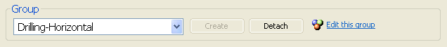
Group: Wells may be added to Well Groups using this pane, either by including them in an existing group (selected from the dropdown list on the left) or by creating it with the Create button. When a group is selected the data is no longer editable in this tab but can be accessed via the corresponding Wells Group node (use the  Edit this group link). Conversely, use the Detach button to remove the well from the group and edit its details in this tab.
Primary-
and Secondary-Fluid Curves
When defining the performance or decline of a well, you must actually provide three different curves: that of the primary fluid (Oil or Gas, depending on the kind of reservoir) and those of the secondary fluids that complete the three-phase (Gas or Oil, and Water).
Secondary-fluid curves are always defined in relation with the primary curve. In the case of Water for  oil reservoirs, the Water Cut means the ratio of Water as a factor of Total Liquid. Gas as secondary fluid in oil reservoirs is computed as GOR (Gas-Oil Ratio, i.e. amount of Gas per volume of Oil).
In  gas reservoirs, Water is expressed as Water Yield, meaning amount of Water per volume of Gas; and Oil as secondary fluid is computed as Oil Yield (amount of Oil per volume of Gas).
See Constant Total Liquid Rate.
Performance Types
PetroVR offers a variety of methods to describe well performance. A main distinction between performance types is that which separates dimensionless types, where factors that will modify a few parameters (Initial Rate, GOR, Well Reserves) are entered, and dimensional, where actual values expressed in units of production and time are used. Dimensionless curves allow more flexibility in modeling, since introducing changes will require only a minimum of steps; e.g., simply modifying Initial Rate will generate a new decline curve of the same shape.
How do I convert my production data to the correct performance format?
Some of these performance types are specific to the kind of well, as shown in the table below:
| Performance Type |  Oil producer Oil producer
|  Gas producer Gas producer
|  Water Injector Water Injector Gas Injector Gas Injector
| CO2 Injection | |
|---|---|---|---|---|---|
Dimensionless | Exponential, Hyperbolic and Harmonic |  | | ||
| Exponential, Hyperbolic and Harmonic | | | |||
| | ||||
| Function Performance Type | | | | ||
| Deliverability (Performance Type) | | ||||
| Quadratic Pressure | | ||||
| Custom Performance Type | | ||||
(either) | | | | ||
Dimensional | Constant Performance Type | |
 Link to Excel: Use this option to dynamically read the decline data from a range of cells in a separate MS Excel worksheet. (When so defined, this button will appear thus: Clear link to Excel.) Read more on this under Working with Tables. Only available for table-formatted performance types: Custom Performance Type and Table Performance Type.
Another option, not visible at first in the Well Performance tab, is to define a performance as Selectable to refer it to a distribution among performance groups already created.
Note also that when switching from one decline to another PetroVR tries to preserve as much of the already entered data as possible. In some cases (e.g., going from a Table Performance Type to Exponential, Hyperbolic and Harmonic) the data formats themselves may be incompatible so that the conversion will not be carried out.
The Well Performance tab of producers and gas injector will be disabled if shared performance options are enabled in the reservoir Well Communication Tab.
The table performance type supports any number of initial rows with 0 as their rate or cum values. The system will simply ignore these rows and interpret them as a time lag intended to align productions profiles in Excel.